The clock-offset problem
I was recently faced with a time-synchronisation problem between two machines. One of the machines, which I will call the server, exposes an endpoint that returns its current time in microseconds. The goal is to measure client-side events in "server time".
The first thing I tried was to synchronise the client using NTP and chrony. However, there was always some offset between the server clock and the client clock. This can happen even when the client is accurately synchronised to its time source, because the server may set its time using a different or private clock. In other words, this is not quite the same problem as synchronising the client to UTC: I need to estimate the relationship between the client clock and the server's application clock.
I observed this offset to be on the order of milliseconds. Existing time-synchronisation protocols are good enough for most applications, where some offset is tolerable, but in this case I would like to measure events in server time with sub-millisecond accuracy. This accuracy depends on the precision of the timestamp returned by the endpoint and on knowing when during request processing the server samples its clock.
Measuring offset from a round trip
My proposed approach is to estimate the clock offset directly and independently of NTP. Every second, I poll the server's time endpoint. For request $k$, let
- $t_{0,k}$ be the client timestamp recorded immediately before sending the request;
- $t_{s,k}$ be the timestamp returned by the server; and
- $t_{1,k}$ be the client timestamp recorded when the response is received.
The observed round-trip time is
$$ d_k = t_{1,k} - t_{0,k}. $$
This duration contains three components: the outbound network delay, the server's processing time, and the inbound network delay. Sampling the clock is effectively instantaneous, but the point during server processing at which $t_{s,k}$ is sampled matters.
If the outbound and inbound delays are approximately equal, the server timestamp corresponds approximately to the client-side midpoint of the request:
$$ m_k = \frac{t_{0,k} + t_{1,k}}{2}. $$
Defining the offset as “server time minus client time,” one measurement of the offset is therefore
$$ z_k = t_{s,k} - m_k = t_{s,k} - \frac{t_{0,k} + t_{1,k}}{2}. $$
The minimum-RTT heuristic
The naive strategy is to retain the offset measurement $z_k$ associated with the request that had the smallest round-trip time over a rolling window. The idea is that this request probably experienced the least queueing delay. This does not mean choosing the smallest offset, which would incorrectly bias the result towards zero.
Minimum round-trip time is only a heuristic. A short request does not guarantee that its outbound and inbound delays were equal. The selected estimate also changes abruptly whenever a faster request arrives or the previous minimum leaves the rolling window. The resulting offset estimate therefore jumps around, which motivates looking for an estimator that can combine noisy measurements over time.
In this article, I investigate whether a Kalman filter can turn these noisy round-trip measurements into a smoother estimate of the server-to-client clock offset, and compare it with the minimum-RTT heuristic.
The Kalman filter as a predict-correct loop
This section follows Dr Shane Ross's Kalman Filter for Beginners: From Theory to MATLAB Implementation lecture series, particularly Part 2: Estimation and Prediction Process. Rather than deriving the filter from first principles, I want to build enough intuition to understand what each equation contributes.
A Kalman filter maintains two things: an estimate of a hidden state and a measure of how uncertain that estimate is. At every time step, it combines two imperfect sources of information:
- a prediction made by a model of how the system behaves; and
- a new, noisy measurement of that system.
The model and the measurement will rarely agree exactly. The filter uses their uncertainties to decide how far the estimate should move towards the new measurement. This produces a repeating predict-correct loop:
$$ \underbrace{(\hat{x}_{k-1}, P_{k-1})}_{\text{previous estimate}} \xrightarrow{\text{predict}} \underbrace{(\hat{x}_k^{-}, P_k^{-})}_{\text{prior}} \xrightarrow{\text{correct using }z_k} \underbrace{(\hat{x}_k, P_k)}_{\text{posterior}}. $$
State and uncertainty
The true state at time step $k$ is $x_k$, while $\hat{x}_k$ is our estimate of it. The state may contain a single value or several related quantities, so in general it is an $n \times 1$ column vector.
An estimate on its own is not enough: we also need to describe how uncertain we are about it. Let $z_{1:k}=(z_1,z_2,\ldots,z_k)$ denote every measurement received up to and including time step $k$. Under the standard linear-Gaussian model, our uncertainty after processing those measurements is written as
$$ x_k \mid z_{1:k} \sim \mathcal{N}\left(\hat{x}_k, P_k\right). $$
The vertical bar means “given.” In words: given measurements $z_1$ through $z_k$, the true state is modelled by a normal distribution with mean $\hat{x}_k$ and covariance $P_k$. The matrix $P_k$ is the covariance of the state-estimation error; it describes the spread of the multidimensional Gaussian distribution around the estimate.
The pair $(\hat{x}_k,P_k)$ is therefore the useful output of the filter: $\hat{x}_k$ says where we think the state is, and $P_k$ says how confident we are in that answer.
Modelling the state and measurement
A standard Kalman filter assumes that the system can be represented by two linear equations. The state equation describes how the hidden state evolves:
$$ x_k = \underbrace{A x_{k-1}}_{\text{linear state transition}} {}+ \underbrace{w_k}_{\text{process noise}}. $$
The measurement equation describes how the hidden state produces an observation:
$$ z_k = \underbrace{H x_k}_{\text{ideal measurement}} {}+ \underbrace{\varepsilon_k}_{\text{measurement noise}}. $$
The matrix $A$ advances the state from one time step to the next. The matrix $H$ maps that state into measurement space: it expresses which parts or combinations of the state a sensor can observe.
The process noise $w_k$ accounts for changes that the state-transition model does not explain. The measurement noise $\varepsilon_k$ accounts for imperfections in the observation itself. The standard model treats both as zero-mean Gaussian noise:
$$ w_k \sim \mathcal{N}(0,Q), \qquad \varepsilon_k \sim \mathcal{N}(0,R). $$
Thus, $Q$ describes uncertainty in the model and $R$ describes uncertainty in the measurements. These are different from $P_k$, which describes uncertainty in the filter's state estimate.
The dimensions of the quantities have to agree:
- $x_k$, $\hat{x}_k$, and $w_k$ are $n \times 1$ state vectors;
- $z_k$ and $\varepsilon_k$ are $m \times 1$ measurement vectors;
- $A$ and $Q$ are $n \times n$ matrices;
- $H$ is an $m \times n$ matrix; and
- $R$ is an $m \times m$ matrix.
Prediction
Suppose the filter has already processed measurement $z_{k-1}$ and holds the estimate $\hat{x}_{k-1}$ with covariance $P_{k-1}$. Before measurement $z_k$ arrives, it uses the state-transition model to predict the state:
$$ \hat{x}_k^{-}=A\hat{x}_{k-1}. $$
The superscript $-$ marks this as the a priori estimate: it is what the filter believes before incorporating the new measurement. The covariance of this prior estimate, $P_k^{-}$, is propagated alongside the state estimate:
$$ P_k^{-} = A P_{k-1} A^\mathsf{T} {}+ \underbrace{Q}_{\text{process-noise covariance}}. $$
The product $A P_{k-1}A^\mathsf{T}$ carries the previous uncertainty through the state-transition model. Adding $Q$ expresses the idea that uncertainty should grow while predicting: the model cannot account perfectly for everything that may happen between two measurements.
At this point the filter has a prior estimate $(\hat{x}_k^{-},P_k^{-})$, but it has not yet used $z_k$.
Correction
When the new measurement arrives, the filter first asks what it expected to measure. Applying $H$ to the predicted state gives $H\hat{x}_k^{-}$. The difference between the actual and predicted measurements is called the innovation or measurement residual:
$$ y_k = \underbrace{z_k}_{\text{measurement}} {}- \underbrace{H\hat{x}_k^{-}}_{\text{predicted measurement}}. $$
If $y_k$ is close to zero, the measurement agrees with the prediction. A large value indicates that the model and measurement disagree, but it does not by itself tell the filter which one is more trustworthy. That decision is encoded by the Kalman gain:
$$ K_k = P_k^{-}H^\mathsf{T} \left(H P_k^{-}H^\mathsf{T}+R\right)^{-1}. $$
The gain compares uncertainty in the predicted state with uncertainty in the measurement. A large $R$ makes the filter cautious about moving towards the measurement. Greater uncertainty in the prediction generally gives the measurement more influence.
The state estimate is corrected by applying this gain to the innovation:
$$ \hat{x}_k = \hat{x}_k^{-} {}+ K_k \left( \overbrace{ \underbrace{z_k}_{\text{measurement}} - \underbrace{H\hat{x}_k^{-}}_{\text{predicted measurement}} }^{\text{innovation }y_k} \right). $$
Finally, the filter updates the state-estimation error covariance:
$$ \begin{aligned} P_k &= (I-K_kH)P_k^{-} \\ &= P_k^{-}-K_kHP_k^{-}. \end{aligned} $$
Here, $I$ is the identity matrix. When a useful measurement is incorporated, the updated covariance will generally be smaller than the prior covariance: the filter has learned something and should be more certain than it was before the correction.
The resulting pair $(\hat{x}_k,P_k)$ is the posterior estimate. It becomes the starting point for the next prediction, and the same cycle repeats for every new measurement.
Choosing the model and initial values
The Kalman equations do not discover the model automatically. To construct a filter, we have to select or estimate four model parameters:
- $A$ - state-transition matrix;
- $H$ - state-to-measurement matrix;
- $Q$ - process-noise covariance; and
- $R$ - measurement-noise covariance.
The filter also needs an initial state:
- $\hat{x}_0$ - initial state estimate; and
- $P_0$ - initial estimation-error covariance.
The values of $Q$ and $R$ determine the balance between prediction and measurement. Setting $Q$ too low makes the filter reluctant to follow changes that are missing from the model. Setting it too high makes the predicted state uncertain. Setting $R$ too low makes the filter chase measurement noise, while setting it too high causes the filter to ignore useful measurements.
Neither covariance matrix has to be diagonal. For zero-mean process noise, an entry of $Q$ is
$$ Q_{ij} = \operatorname{Cov}\left(w_k^{(i)},w_k^{(j)}\right). $$
What does Cov mean, and how is it computed?
The complete process-noise term \(w_k\) is a random vector. Its covariance is therefore the matrix
Each matrix entry compares two scalar components of that vector. In other words, \(w_k^{(i)}\) and \(w_k^{(j)}\) are scalar random variables, and
Here, \(E[\cdot]\) denotes the expected, or average, value. Because the Kalman model assumes zero-mean process noise, each entry simplifies to
Given \(N\) observed noise samples, the covariance can be estimated using the sample covariance
Process noise is often not directly observable. If the true states were known, we could obtain it from \(w_k=x_k-Ax_{k-1}\). In practice, \(Q\) is commonly derived from a physical model, estimated from historical data, or treated as a tuning parameter.
Let $\sigma_i$ denote the standard deviation of the $i$-th process-noise component, $w_k^{(i)}$. Its variance is the square of that standard deviation:
$$ \operatorname{Var}\left(w_k^{(i)}\right) = \operatorname{Cov}\left(w_k^{(i)},w_k^{(i)}\right) = \sigma_i^2. $$
The diagonal entries of $Q$ are these individual variances, while the off-diagonal entries describe how two different noise components vary together. If the process-noise components are uncorrelated, the off-diagonal entries are zero and $Q$ is diagonal:
$$ Q = \begin{bmatrix} \sigma_1^2 & 0 & \cdots & 0 \\ 0 & \sigma_2^2 & \cdots & 0 \\ \vdots & \vdots & \ddots & \vdots \\ 0 & 0 & \cdots & \sigma_n^2 \end{bmatrix}. $$
The same reasoning applies to $R$: it is diagonal when the components of the measurement noise are uncorrelated. Diagonal matrices are often a useful starting assumption, but the assumption should come from the noise model rather than being imposed by the Kalman filter.
Algorithm summary
Once $A$, $H$, $Q$, and $R$ have been specified, the discussion above reduces to a short recursive algorithm. Start by choosing the initial estimate $\hat{x}_0$ and its covariance $P_0$. Then, for each new measurement $z_k$, perform the following steps.
-
Predict the state and its covariance:
$$ \begin{aligned} \hat{x}_k^{-} &= A\hat{x}_{k-1}, \\ P_k^{-} &= A P_{k-1}A^\mathsf{T}+Q. \end{aligned} $$
-
Compute the innovation $y_k$ and its covariance $S_k$:
$$ \begin{aligned} y_k &= z_k-H\hat{x}_k^{-}, \\ S_k &= H P_k^{-}H^\mathsf{T}+R. \end{aligned} $$
-
Compute the Kalman gain:
$$ K_k=P_k^{-}H^\mathsf{T}S_k^{-1}. $$
-
Correct the state estimate:
$$ \hat{x}_k=\hat{x}_k^{-}+K_k y_k. $$
-
Correct the state-estimation error covariance:
$$ P_k=(I-K_kH)P_k^{-}. $$
The corrected pair $(\hat{x}_k,P_k)$ becomes the input to the prediction step when measurement $z_{k+1}$ arrives. In this way, the filter retains everything it has learned so far using only the current estimate and covariance rather than the complete measurement history.
These definitions are abstract on their own, so the next section constructs $A$, $H$, $Q$, and $R$ for a concrete system.
A simple physical example - estimating altitude and velocity
The equations in the previous section become more concrete once every term is attached to a physical quantity. In Dr Shane Ross's example, we have 1,501 sonar measurements of altitude in metres, sampled every $0.01$ seconds. The sonar observes altitude directly, but we would also like to estimate the point's vertical velocity.
Taking the difference between consecutive measurements might appear to give us velocity. In practice, differentiation also amplifies measurement noise. The largest one-sample change in this dataset is approximately $-14.7$ metres; dividing it by $0.01$ seconds would produce an implausible velocity of about $-1474$ metres per second. Instead, we will estimate velocity as part of the hidden state and let the Kalman filter combine evidence over time.
Choosing the state-transition model
We represent the state using altitude $p_k$ and vertical velocity $v_k$:
$$ x_k = \begin{bmatrix} p_k \\ v_k \end{bmatrix}. $$
Between measurements, our best guess is that the current velocity remains unchanged. We have no information telling us that it should systematically increase or decrease, so assuming either would introduce an acceleration that we have no evidence for:
$$ \begin{aligned} p_{k+1} &= p_k + v_k\Delta t, \\ v_{k+1} &= v_k. \end{aligned} $$
In matrix form, the state equation is
$$ \begin{aligned} x_{k+1} &= \underbrace{ \begin{bmatrix} 1 & \Delta t \\ 0 & 1 \end{bmatrix} }_{A} x_k {}+ w_k. \end{aligned} $$
For $\Delta t=0.01$ seconds, this gives
$$ A = \begin{bmatrix} 1 & 0.01 \\ 0 & 1 \end{bmatrix}. $$
This does not assert that the real velocity is physically constant. It is the prediction we make in the absence of new evidence. Acceleration and other departures from that prediction are represented by the process-noise term $w_k$.
Following the example values introduced above, we choose
$$ Q = \begin{bmatrix} 1 & 0 \\ 0 & 3 \end{bmatrix}. $$
The entry $Q_{22}=3$ gives the velocity component non-zero process variance, so the filter can revise velocity rather than treating the constant-velocity prediction as exact. The values $1$ and $3$ should not be compared as though they had the same units: $Q_{11}$ is a position variance and $Q_{22}$ is a velocity variance. This $Q$ is an initial tuning choice, not a covariance derived from a physical acceleration model or calibrated for this sonar.
Connecting the state to the sonar
Each sonar observation contains altitude but no velocity. The measurement matrix must therefore select the first component of the state:
$$ \begin{aligned} z_k &= Hx_k + \varepsilon_k \\[4pt] &= \underbrace{ \begin{bmatrix} 1 & 0 \end{bmatrix} }_{H} \begin{bmatrix} p_k \\ v_k \end{bmatrix} {}+ \varepsilon_k \\[4pt] &= p_k + \varepsilon_k. \end{aligned} $$
We use $\varepsilon_k$ for measurement noise to distinguish it from the velocity $v_k$, and model it as
$$ \varepsilon_k \sim \mathcal{N}(0,R). $$
For this example, we choose a measurement-noise variance of
$$ R=10\ \mathrm{m}^2. $$
This corresponds to a measurement-noise standard deviation of $\sqrt{10}\approx3.16$ metres. A larger $R$ means that we consider the sonar measurements less reliable. This reduces the Kalman gain, so each correction stays closer to the model's prediction. A smaller $R$ expresses greater trust in the sonar and gives each measurement more influence over the corrected estimate.
Initializing the filter
The model is now defined by $A$, $H$, $Q$, and $R$, but the recursive algorithm also needs a starting estimate. We use the first sonar measurement $z_0$ as the initial altitude and initially assume zero vertical velocity:
$$ \hat{x}_0 = \begin{bmatrix} z_0 \\ 0 \end{bmatrix}. $$
The first altitude estimate came from a noisy measurement, while the initial velocity is completely unobserved. We express that difference using
$$ P_0 = \begin{bmatrix} 10 & 0 \\ 0 & 100 \end{bmatrix}. $$
Here, the initial altitude variance matches $R$, while the larger velocity variance lets the early measurements correct our arbitrary initial velocity quickly. These initial values are part of the model and should be revisited when more prior information is available.
Running the predict-correct loop
Since $z_0$ initialized the state, the recursive loop begins with the second measurement. At every step, we predict $(\hat{x}_k^-,P_k^-)$, compare the predicted altitude with the new sonar observation, compute the Kalman gain, and produce the corrected pair $(\hat{x}_k,P_k)$. That posterior becomes the input to the next prediction.
I implemented and ran this loop in an executable Jupyter notebook. The notebook contains the complete Python implementation, its saved output, and a link for running it in Google Colab.
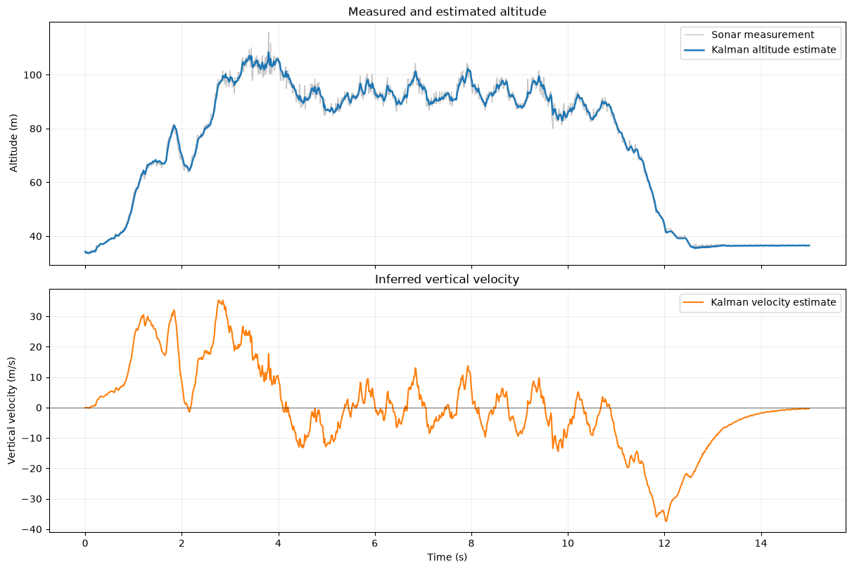
The upper plot compares the sonar observations with the posterior altitude estimate. The lower plot shows the vertical velocity inferred by the filter: positive values correspond to increasing altitude and negative values to decreasing altitude.
There is no ground-truth altitude or velocity in the dataset, so this result does not prove that the estimates are accurate. It shows how the constant-velocity model and the chosen $Q$ and $R$ interpret the measurements. Tuning those covariances - and eventually deriving them from the sensor and motion model - is part of turning this illustrative filter into a reliable estimator.
Returning to the clock-offset problem
The altitude example began with a physical model and then selected a state, $A$, $H$, $Q$, and $R$ to describe it. I can now do the same for the clock measurements from the beginning of the article.
My first attempt used a scalar Kalman filter whose only state was one constant offset. That model worked on simulated measurements with a fixed true offset, but it was too rigid for the real recording. Across approximately 24 hours, the midpoint observations move between several relatively stable levels and also change gradually within those periods. A filter forced to learn one constant would eventually become very confident in an average of the past. That average would not describe the offset at the time of a new event.
The objective is therefore slightly different from the one I started with. I am not trying to find one offset for the complete recording. I want an online estimate of the current offset which is smooth enough to reject individual network-delay fluctuations but responsive enough to follow a sustained change.
What the state represents
For this model I use a three-component state:
$$ x_k = \begin{bmatrix} o_k \\ \rho_k \\ \beta_k \end{bmatrix}. $$
Each component has a separate role:
- $o_k$ is the current effective low-delay offset in microseconds. As before, the sign convention is server time minus client time. A positive value means that the server clock is ahead; a negative value means that the client clock is ahead.
- $\rho_k$ is the background rate at which the offset changes, measured in microseconds per second. Numerically, this is also parts per million.
- $\beta_k$ describes an empirical relationship between request RTT and the midpoint offset measurement. It is measured in microseconds of apparent offset per additional microsecond of RTT.
I call $o_k$ an effective offset because the three timestamps do not isolate the two clocks perfectly. The midpoint calculation also contains any persistent difference between the outbound and inbound path delays. A change in $o_k$ might therefore be caused by a clock correction, a change in path asymmetry, or some combination of the two. The filter cannot distinguish between those explanations.
Predicting the state
Let $\Delta t_k$ be the elapsed time in seconds since the previous measurement. In the absence of a new observation, the model predicts that the offset continues at the current drift rate, while the drift and RTT coefficient remain unchanged:
$$ x_k^- = A_k x_{k-1}, \qquad A_k = \begin{bmatrix} 1 & \Delta t_k & 0 \\ 0 & 1 & 0 \\ 0 & 0 & 1 \end{bmatrix}. $$
Multiplying out the first row gives
$$ o_k^- = o_{k-1} + \rho_{k-1}\Delta t_k. $$
This is the clock equivalent of the position and velocity prediction in the sonar example. The offset plays the role of position and the drift plays the role of velocity. The matrix $A_k$ says how the three state components evolve between measurements; it does not say how they are observed.
The real measurements do not follow a constant-drift line exactly. I allow the effective offset to move away from that prediction using
$$ x_k = A_kx_{k-1}+w_k, \qquad w_k\sim\mathcal N(0,Q_k), $$
with
$$ Q_k = \begin{bmatrix} \sigma_o^2\Delta t_k & 0 & 0 \\ 0 & 0 & 0 \\ 0 & 0 & 0 \end{bmatrix}. $$
Only the offset receives process noise. This is the random-walk part of the model. It is not a claim that either physical clock jumps randomly every second. It is a statistical allowance for changes which the constant-drift prediction cannot explain. Multiplication by $\Delta t_k$ also means that the filter becomes appropriately less certain after a longer gap between measurements.
The prediction covariance is
$$ P_k^- = A_kP_{k-1}A_k^\mathsf{T}+Q_k. $$
Here, $P_k^-$ is the filter's uncertainty about the predicted state. Adding $Q_k$ prevents that uncertainty, and consequently the Kalman gain, from collapsing towards zero after a long sequence of observations. This is what lets sustained new evidence move the estimate towards a new offset level.
Connecting RTT to the observation
The raw observation is still the midpoint estimate
$$ z_k=t_{s,k}-\frac{t_{0,k}+t_{1,k}}{2}. $$
In this dataset, slower requests tend to produce systematically higher midpoint observations. Merely increasing $R$ for a slow request would give it less influence, but would not account for that systematic shift. I therefore model the observation as
$$ z_k = o_k+\beta_k(d_k-d_{\mathrm{base}})+\varepsilon_k. $$
The value $d_{\mathrm{base}}$ is a low reference RTT. I use the 0.1 percentile of observed RTTs rather than the single minimum, making the reference less sensitive to one exceptional sample. In the current recording it is approximately $426\,\mu\mathrm{s}$. The state component $o_k$ should therefore be read as the effective offset for a request close to that low-delay baseline.
For example, if $\beta_k=0.2$ and a request takes $100\,\mu\mathrm{s}$ longer than $d_{\mathrm{base}}$, the model expects its midpoint observation to be $20\,\mu\mathrm{s}$ higher. The coefficient does not recover the outbound and inbound delays. It learns only the linear relationship visible in these measurements.
The same observation equation can be written in standard Kalman notation:
$$ z_k=H_kx_k+\varepsilon_k, \qquad H_k= \begin{bmatrix} 1 & 0 & d_k-d_{\mathrm{base}} \end{bmatrix}. $$
The first entry of $H_k$ selects the current offset. The zero means that one request does not observe drift directly; the filter infers drift from changes across many requests. The final entry connects excess RTT to $\beta_k$. Since each request produces one scalar offset observation, $H_k$ has one row.
I model the remaining measurement error as
$$ \varepsilon_k\sim\mathcal N(0,R_k), \qquad R_k=(50\,\mu\mathrm{s})^2. $$
Thus, $R_k$ expresses the residual scatter I expect after accounting for the linear RTT effect. A larger value would make each request move the estimate less; a smaller value would make the filter follow individual observations more closely. I also exclude the slowest five percent of requests because their errors are not described well by this simple linear relationship. That cutoff is a modelling choice, not a requirement of the Kalman filter.
Together, the four matrices now have concrete meanings:
- $A_k$ advances offset using the estimated clock drift;
- $H_k$ predicts the midpoint observation for the request's RTT;
- $Q_k$ permits the effective offset to depart from constant drift; and
- $R_k$ describes the remaining uncertainty in one midpoint observation.
The usual predict-correct equations from the primer can then be applied without modification. Although $A_k$ and $H_k$ change with $\Delta t_k$ and $d_k$, the model remains linear in the hidden state.
Choosing how quickly the filter follows a change
The value $\sigma_o$ in $Q_k$ controls the compromise I care about most. A small value produces a smooth estimate but takes longer to follow a new offset level. A large value reacts quickly but allows more measurement noise into the estimate.
I tested several candidate values using one-step-ahead prediction. Each candidate processed the first 75 percent of the recording sequentially, and I also checked its prediction score on the remaining 25 percent. This selected
$$ \sigma_o=1.5\,\mu\mathrm{s}/\sqrt{\mathrm{s}}. $$
With the measurements arriving approximately once per second, the median offset component of the Kalman gain is about $0.03$. Its reciprocal gives a rough response scale of 33 accepted observations. This is not an exact settling time, but it conveys the intended behaviour: one unusual request has little effect, while a new level supported by tens of observations moves the estimate substantially.
What the recording shows
The complete implementation and its executed output are available in an accompanying Jupyter notebook.
The clock-measurement dataset currently contains 88,445 requests spanning about 24.6 hours. After excluding the slowest five percent, the filter processes 84,022 observations. The learned RTT coefficient is approximately $0.289$, meaning that an additional $100\,\mu\mathrm{s}$ of RTT is associated with about $28.9\,\mu\mathrm{s}$ of upward shift in the midpoint observation.
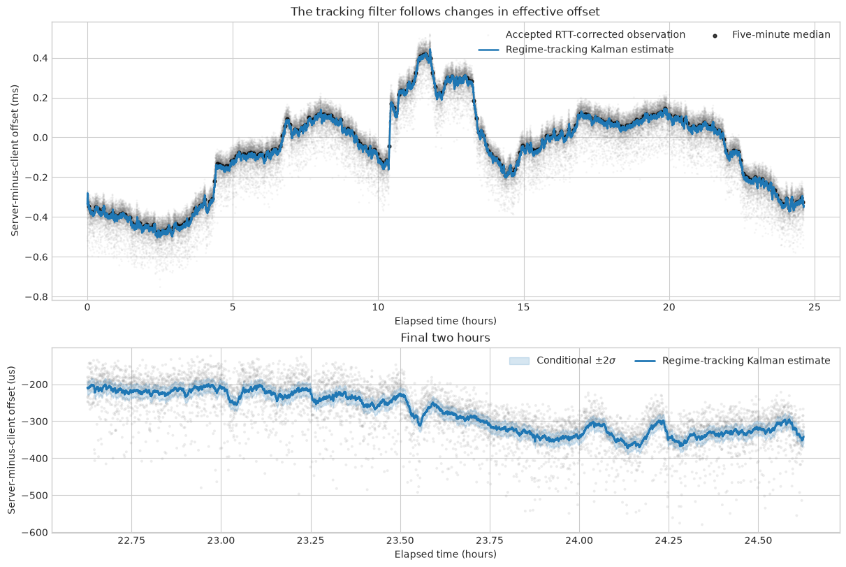
The grey points are accepted observations after applying the learned linear RTT correction. The blue curve is the posterior estimate of the effective low-delay offset. The black points are five-minute medians of the corrected observations and provide a robust visual reference. They are not independent ground truth because they come from the same measurements.
Most importantly, the blue curve does not converge to one value for the complete recording. It follows gradual changes and several sharper transitions while remaining much smoother than the individual requests. The filter does not explicitly detect regime boundaries or assign a constant to each regime. Instead, it continuously estimates the local offset. Relatively stable stretches of that trajectory are what I refer to informally as regimes.
As an internal tracking diagnostic, the filter's end-of-block estimate differs from the corresponding five-minute median by about $12.4\,\mu\mathrm{s}$ on average, with 95 percent of the absolute differences below approximately $30.5\,\mu\mathrm{s}$. This measures how closely the chosen smoothing follows a reference derived from the same data. It does not demonstrate $30\,\mu\mathrm{s}$ accuracy relative to the true clock offset.
For the same reason, the estimate at the final observation is not a summary of the preceding 24 hours. If I wanted to express an event in server time, I would use the filter estimate at that event's timestamp. In an online system, the latest posterior and covariance would simply be retained as the starting point for the next request.
What this filter can and cannot tell me
The Kalman filter improves the way I combine observations over time. It gives me a smooth, recursive estimate, retains uncertainty, learns the observed RTT effect, and can follow sustained changes instead of averaging them away. It does not create information which the endpoint did not provide.
With only $t_{0,k}$, $t_{s,k}$, and $t_{1,k}$, I observe total round-trip time but not the outbound and inbound delays separately. A fixed path asymmetry is therefore indistinguishable from clock offset. A changing asymmetry can look like a changing clock. The uncertainty reported by $P_k$ is conditional on the linear-Gaussian model and does not include an unknown fixed error from that asymmetry.
Consequently, the result should be described as an estimate of the effective server-minus-client offset under this measurement method, not as a verified measurement of the physical difference between the clocks. Testing absolute accuracy would require an independent reference or a protocol which exposes enough timestamps to estimate the two directions separately.
That limitation does not make the filter useless. For translating events consistently into the server's application time, the local offset trajectory is more useful than either a noisy midpoint measurement or the minimum-RTT sample from a rolling window. The important conclusion is not that the Kalman filter discovers one true constant. It is that a carefully chosen state and noise model turn a stream of imperfect round trips into a stable estimate which can still adapt when the observed timing relationship changes.